Chemical dissolution
Rationale
The details could be found in paper by [11].
Limestone is made of $CaCO_3$, and it is easily dissolved. Limestone's dissolution mainly depends on precipitation (rainfall) and temperature. The paper used equation 1 to quantify this process.
\[\frac{dh}{dt} = 0.001\ \kappa_c\ {{q_i} \over {A_i}}\]
Herein $dh/dt$ is the chemical weathering rate and the unit is in m/s. Other parameters are defined as: $q_i$ is the discharge of water at a certain cell. $A_i$ is the surface area of the cell. If we assume there would be no surface water on land, $q_i$ reduces to precipitation – evaporation. For example, we can set it to 400 mm/y for demonstration purposes. Therefore equation 1 could be reduced to Equation 2.
\[\frac{dh}{dt} = 0.001\ \kappa_c\ I\]
Where $I$ is runoff (mm/yr). The parameter $\kappa_c$ is dimensionless and should be described by equation 3:
\[\kappa_c = 40\times 1000\ \frac{[Ca^{2+}]_{eq}}{\rho}\]
Parameter ρ is the density of calcite, and we choose 2700 $kg/m^3$ here for the default value. $[Ca^{2+}]_{eq}$ is defined in equation 4:
\[[Ca^{2+}]_{eq} = {{(PCO_2\ (K_1\ K_C\ K_H)} \over {(4\ K_2\times \gamma Ca\ (\gamma HCO_3)^2)^{(1/3)}}}\]
Mass balance coefficients $K_1$, $K_2$, $K_C$, $K_H$ depend on temperature. $_PCO_2$ is assumed to be between $10^{-1.5} ATM$ to $10^{-3.5} ATM$.
Other parameters can be found in the following table by [11].
| Parameter | Description | Unit | Value |
|---|---|---|---|
| T | Absolute temperature | [°K] | Tc + 273.16 |
| I | Ion activity | [-] | 0.1 |
| $A^*$ | Debye-Hückel coefficient | [-] | $-0.4883 + 8.074 \times 10^{-4}T_c$ |
| $B^*$ | Debye-Hückel coefficient | [-] | $-0.3241 + 1.600 \times 10^{-4}T_c$ |
| $log \gamma Ca\dagger$ | Activity coefficient | [-] | $-4A\sqrt{I}(1 + 5.0 x 10^{-8}B\sqrt{I})$ |
| $log \gamma HCO_3\dagger$ | Activity coefficient | [-] | $-1A\sqrt{I}/(1 + 5.4 x 10^{-8}B\sqrt{I})$ |
| $log K_1\ddagger$ | Mass balance coefficient | [ $mol L^{-1}$ ] | $-356.3094 - 0.06091964T + 21834.37/T + 126.8339logT - 1684915/T^2$ |
| $log K_2\ddagger$ | Mass balance coefficient | [ $mol L^{-1}$ ] | $-107.8871 - 0.03252849T + 5151.79/T + 38.92561logT - 563713.9/T^2$ |
| $log K_c\ddagger$ | Mass balance coefficient | [ $mol^2 L^{-2}$ ] | $-171.9065 - 0.077993T + 2839.319/T + 71.595logT$ |
| $log K_H\ddagger$ | Mass balance coefficient | [ $mol L^{-1} atm^{-1}$ ] | $108.3865 + 0.01985076T - 6919.53/T - 40.45154logT + 669365/T^2$ |
These parameters are calculated from temperature using the karst_denudation_parameters function:
function karst_denudation_parameters(temp::Float64)
A = -0.4883 + 8.074 * 0.0001 * (temp - 273.0)
B = -0.3241 + 1.6 * 0.0001 * (temp - 273.0)
IA = 0.1 # ion activity
(K1=10^(-356.3094 - 0.06091964 * temp + 21834.37 / temp + 126.8339 * log10(temp) - 1684915 / (temp^2)),
K2=10^(-107.881 - 0.03252849 * temp + 5151.79 / temp + 38.92561 * log10(temp) - 563713.9 / (temp^2)),
KC=10^(-171.9065 - 0.077993 * temp + 2839.319 / temp + 71.595 * log10(temp)),
KH=10^(108.3865 + 0.01985076 * temp - 6919.53 / temp - 40.4515 * log10(temp) + 669365 / (temp^2)),
activity_Ca=10^(-4A * sqrt(IA) / (1 + 10^(-8) * B * sqrt(IA))),
activity_Alk=10^(-A * sqrt(IA) / (1 + 5.4 * 10^(-8) * B * sqrt(IA))))
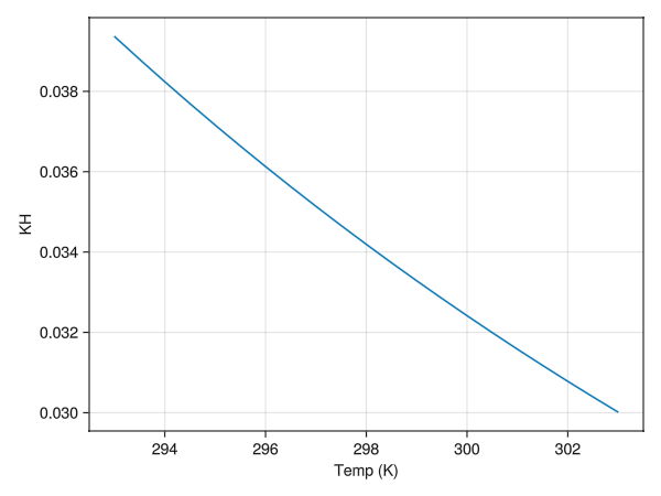
endThe output of this function for the $K_H$ parameter is plotted below for a range of input temperatures
Plotting code
#| requires: examples/denudation/dissolution-test.jl
#| creates:
#| - docs/src/_fig/KHTemp.png
#| - docs/src/_fig/Equilibrium_Concs.png
#| - docs/src/_fig/DissolutionExample.png
#| collect: figures
module DissolutionSpec
using CairoMakie
using Unitful
using CarboKitten.Denudation.DissolutionMod: equilibrium, dissolution, karst_denudation_parameters
using CarboKitten: Box
using CarboKitten.Stencil: Periodic, Reflected, stencil
@kwdef struct facies
infiltration_coefficient :: Float64
mass_density :: typeof(1.0u"kg/m^3")
reactive_surface :: typeof(1.0u"m^2/m^3")
end
@kwdef struct Dissolution
temp :: Any
precip :: Float64
pco2 :: Float64
reactionrate :: Float64
end
@kwdef struct state
ca::Matrix{Int}
end
const BOX = Box{Periodic{2}}(grid_size=(5, 5), phys_scale=1.0u"km")
const Facies = facies(infiltration_coefficient = 0.5,
mass_density = 2.73u"kg/m^3",
reactive_surface = 1000u"m^2/m^3")
const DIS = Dissolution(temp = 285,
precip = 1.0,
pco2 = 10^(-1.5),
reactionrate = 0.1)
const STATE = state(ca =
[ 0 0 1 0 0
0 1 0 1 1
0 0 1 0 1
1 0 1 1 0
1 1 1 1 0])
const WD = -10 .* [ 0.0663001 0.115606 0.646196
0.601523 0.130196 0.390821
0.864734 0.902935 0.670354]
function main()
temp = collect(293:0.5:303)
Eq_result = Array{Any,1}(undef,length(temp))
Para_result = Array{Any,1}(undef,length(temp))
Dis_result = Array{Any,1}(undef,length(temp))
Dis_result_wd = Array{Any,1}(undef,length(WD))
for i in eachindex(temp)
Para_result[i] = karst_denudation_parameters(temp[i])
end
Para_result_KH = [x.KH for x in Para_result]
for i in eachindex(temp)
Eq_result[i] = equilibrium(temp[i],DIS.pco2,DIS.precip,Facies)
end
Eq_result_concs = [x.concentration for x in Eq_result]
for i in eachindex(temp)
Dis_result[i] = dissolution(temp[i],DIS.precip,DIS.pco2,DIS.reactionrate,WD[1],Facies)
end
Dis_result
for i in eachindex(WD)
Dis_result_wd[i] = dissolution(temp[1],DIS.precip,DIS.pco2,DIS.reactionrate,WD[i],Facies)
end
Dis_result_wd
fig1 = Figure()
ax1 = Axis(fig1[1,1],xlabel="Temp (K)", ylabel=" concentration (mol/L)")
lines!(ax1,temp,Eq_result_concs)
save("docs/src/_fig/Equilibrium_Concs.png",fig1)
fig2 = Figure()
ax2 = Axis(fig2[1,1],xlabel="Temp (K)", ylabel="KH")
lines!(ax2,temp,Para_result_KH)
save("docs/src/_fig/KHTemp.png",fig2)
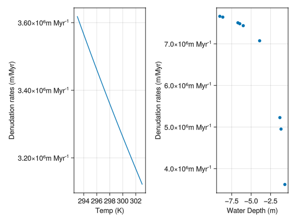
fig3 = Figure()
ax3 = Axis(fig3[1,1],xlabel="Temp (K)", ylabel="Denudation rates (m/Myr)")
lines!(ax3,temp,Dis_result)
ax4 = Axis(fig3[1,2],xlabel="Water Depth (m)", ylabel="Denudation rates (m/Myr)")
scatter!(ax4,vec(WD),Dis_result_wd)
fig3
save("docs/src/_fig/DissolutionExample.png",fig3)
end
end
DissolutionSpec.main()The $[Ca^{2+}]_{eq}$ parameter is calculated from temperature using the equilibrium function:
function equilibrium(temp::Float64, pco2::Float64, precip::Float64, facies)
    p = karst_denudation_parameters(temp)
    mass_density = facies.mass_density ./ u"kg/m^3"
    eq_c = (pco2 .* (p.K1 * p.KC * p.KH) ./ (4 * p.K2 * p.activity_Ca .* (p.activity_Alk)^2)) .^ (1 / 3)
    eq_d = 1e6 * precip .* facies.infiltration_coefficient * 40 * 1000 .* eq_c ./ mass_density
    (concentration=eq_c, denudation=eq_d)
end
The values of $[Ca^{2+}]_{eq}$ are calculated in equilibrium for a range of temperatures: 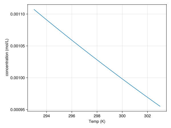
The above discussion is true only if the percolated fluid is saturated (in terms of Ca) when leaving the platform. However, in some cases, the fluid is not saturated when they leave the platform, the dissolved amount is thus lower than the scenario described above.
The following articles describe this: [12] and [13]
Ideally, a reactive transport model (RTMs) is sufficiently accurate to solve this prolem, but employing RTMs needs more computational resources. So herein, the author simplify the process and assumed the dissolution rates of rocks depend on the depth. This is a reasonable assumption, because the deeper the solution penetrates, the more concentrated it becomes. This assumption does not consider diffusion in this chapter.
The dissolution rate of carbonate follows linear rate laws of:
\[F = \alpha (c_{eq}-c(z))\]
The rate law is a common expression way to describe the kinetics of certain chemical reactions see Rate Laws.
\[F\]
is the dissolution rate, $\alpha$ is constant (kinetic co-efficient), $c_{eq}$ is the concentration in fluid when equilibrium is reached (i.e., no more dissolution, which is $[Ca^{2+}]_{eq}$ in Chapter 1), $c(z)$ is the current concentrationion at depth $z$ in the fluid. This equation then expands to
\[I\ {\rm d}c = \alpha (c_{eq}-c(z)) L\ {\rm d}z\]
This equation employs mass balance and indicates that the concentration increase in the infiltrated water equals the dissolution of rocks in the thickness of $dz$. $L$ is the specific length of fractures/porosities (units: $m/m^2$). I.e., this term defines the relative reactive surface of the subsurface rocks, or how much surface is actually undergoing dissolution. This parameter is difficult to obtain in the fields but feel free to adjust it to see how the results would change.
However, to solve this equation we still need to know $c(z)$.
If assuming the initial percolating water has $c(0) = 0$, then we could get the following equation (as $c$ is related to depth):
\[c(z) = c_{eq}\ (1 - e^{(-z/\lambda)})\]
Herein, $ \lambda = {{I} \over {\alpha L}} $.
Therefore,
\[D_{\rm average} = (I\times \frac{c_{eq}}{\rho})\ (1 – (\frac{\lambda}{z_0})\ (1 – e^{(\frac{-z_0}{\lambda})}))\]
α used in the default setting are $\alpha = 2·10^{−6}$ or $3.5·10^{−7}$ cm/s (for temp at 298K). This is indeed a controversial parameter. Please feel free to try different values and see what happens.
These equations are implemented as dissolution function:
function dissolution(temp, precip, pco2, alpha, water_depth, facies)
    reactive_surface =  facies.reactive_surface ./u"m^2/m^3"
    λ = precip * 100 .* facies.infiltration_coefficient ./ (alpha .* reactive_surface)
    eq = equilibrium(temp, pco2, precip, facies) # pass ceq Deq from the last function
    eq.denudation .* (1 - (λ ./ -water_depth) .* (1 - exp.(water_depth ./ λ))) * u"m/Myr"
end
The dedudation rates calculated from this function for varying temperature and water depth are plotted here:
Implementation
module DissolutionMod

import ..Abstract: DenudationType, denudation, redistribution
using ...BoundaryTrait: Boundary
using ...Boxes: Box
export Dissolution
using Unitful

@kwdef struct Dissolution <: DenudationType
    temp::typeof(1.0u"K")
    precip::typeof(1.0u"m/yr")
    pco2::typeof(1.0u"atm")
    reactionrate::typeof(1.0u"m/yr")
end

<<karst-parameter-function>>

#calculate ceq and Deq, Kaufman 2002
<<karst-equilibrium-function>>

<<karst-dissolution-function>>


function denudation(::Box{BT}, p::Dissolution, water_depth, slope, facies, state) where {BT<:Boundary}
    temp = p.temp ./ u"K"
    precip = p.precip ./ u"m/yr"
    pco2 = p.pco2 ./1.0u"atm"
    reactionrate = p.reactionrate ./u"m/yr"
    denudation_rate = zeros(typeof(1.0u"m/Myr"), length(facies), size(state.ca)...)

    for idx in CartesianIndices(state.ca)
        f = state.ca[idx]
        if f == 0
            continue
        end
        if water_depth[idx] <= 0
            denudation_rate[f, idx] = dissolution(temp, precip, pco2, reactionrate, water_depth[idx], facies[f])
        end
    end
    return denudation_rate
end

function redistribution(box::Box{BT}, p::Dissolution, denudation_mass, water_depth) where {BT<:Boundary}
    return nothing
end

end
Result example
The resultant figures of chemical dissolution is presented below: 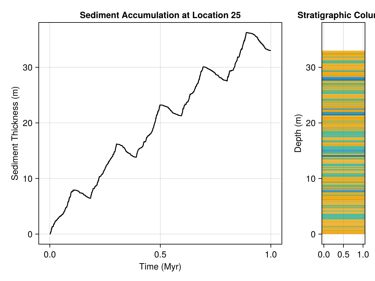
We can clearly see the sediments were removed as the thickness of sediments decrease at each regression cycle.