Physical erosion and sediment redistribution

Rationale

This approach not only considers the amount of materials that have been physically removed, but also how the eroded materials are being distributed to the neighboring regions depending on slopes on each direction.

Physical erosion

The equations used to estimate how much material could one cell provide to the neighboring topographically lower cells is described below. The equation is found in [14]. We choose this equation mainly because it specifically deals with bedrock substrates instead of loose sediments. In the equation, $k_v$ is erodibility, and the default value is 0.0023 according to the paper. $(1 - I_f)$ indicates run-off generated in one cell and slope is the slope calculated based on ArcGis: how slope works. Note that the algorithms to calculate slope does not work on enclosed depressions.

\[D_{phys} = -k_v \times (1 - I_f)^{1/3} |\nabla h|^{2/3}\]

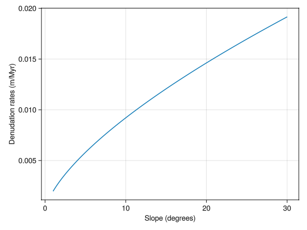
This equation for the physical dedundation rate, $D_{phys}$ is implemented in code as follows:

function physical_erosion(slope::Float64, inf::Float64, erodibility::Any)
    -1 * -erodibility .* (1 - inf) .^ (1 / 3) .* slope .^ (2 / 3)
end

and the output of this function for a range of slope angles is plotted here:

#| requires: examples/denudation/physical-test.jl
#| creates: docs/src/_fig/PhysicalSlope.png
#| collect: figures
module PhysicalSpec

using CairoMakie
using CarboKitten.Denudation.EmpiricalDenudationMod: slope_kernel
using CarboKitten.Denudation.PhysicalErosionMod: physical_erosion, redistribution_kernel
using CarboKitten.Stencil: Boundary, Periodic, offset_value, offset_index, stencil
using CarboKitten.BoundaryTrait
import CarboKitten.Config: Box

const inf = 0.5
const erodibility = 0.0025

function main()
    SLOPE = collect(1:0.2:30)
    DEN_MASS = Vector{Float64}(undef,size(SLOPE))

    for i in eachindex(SLOPE)
        DEN_MASS[i] = physical_erosion(SLOPE[i],inf,erodibility)
    end

    w = 10 .* [ 0.0663001  0.115606  0.646196
    0.601523   0.130196  0.390821
    0.864734   0.902935  0.670354]

    fig = Figure()
    ax = Axis(fig[1,1],xlabel="Slope (degrees)", ylabel="Denudation rates (m/Myr)")
    lines!(ax,SLOPE,DEN_MASS)
    save("docs/src/_fig/PhysicalSlope.png",fig)
end

end

PhysicalSpec.main()

Redistribution of sediments

The redistribution of sediments after physical erosion is based on [15]: the eroded sediments calculated using the above equation are distributed to the neighboring 8 cells according to the slopes (defined as elevation differences/horizontal differences) towards each direction. The details of calculating the amount of sediments of one cell received are presented in the following section.

Implementation

module PhysicalErosionMod

import ..Abstract: DenudationType, denudation, redistribution
using ...Stencil: Boundary, Periodic, offset_value, offset_index, stencil
using ...BoundaryTrait
using ...Boxes: Box

using Unitful

@kwdef struct PhysicalErosion <: DenudationType end

const Amount = typeof(1.0u"m")

<<physical-erosion>>

function redistribution_kernel(w::Array{Float64}, cellsize::Float64)
    s = zeros(Float64, (3, 3))
    s[1, 1] = (w[1, 1] - w[2, 2]) / cellsize
    s[1, 2] = (w[1, 2] - w[2, 2]) / cellsize / sqrt(2)
    s[1, 3] = (w[1, 3] - w[2, 2]) / cellsize
    s[2, 1] = (w[2, 1] - w[2, 2]) / cellsize / sqrt(2)
    s[2, 2] = (w[2, 2] - w[2, 2]) / cellsize
    s[2, 3] = (w[2, 3] - w[2, 2]) / cellsize / sqrt(2)
    s[3, 1] = (w[3, 1] - w[2, 2]) / cellsize
    s[3, 2] = (w[3, 2] - w[2, 2]) / cellsize / sqrt(2)
    s[3, 3] = (w[3, 3] - w[2, 2]) / cellsize

    s[s.<0.0] .= 0.0
    sumslope = sum(s)

    if sumslope == 0.0
        return zeros(Float64, (3, 3))
    else
        return s ./ sumslope
    end
end

function mass_erosion(box::Box{BT}, denudation_mass, water_depth::Array{Float64}, i::CartesianIndex) where {BT<:Boundary{2}}
    wd = zeros(Float64, 3, 3)
    for (k, Δi) in enumerate(CartesianIndices((-1:1, -1:1)))
        wd[k] = offset_value(BT, water_depth, i, Δi)
    end
    cell_size = box.phys_scale ./ u"m"

    return (redistribution_kernel(wd, cell_size) .* denudation_mass[i])
end

function total_mass_redistribution(box::Box{BT}, denudation_mass, water_depth, mass) where {BT<:Boundary{2}}
        for i in CartesianIndices(mass)
            redis = mass_erosion(box, denudation_mass, water_depth, i)

            for subidx in CartesianIndices((-1:1, -1:1))
                target = offset_index(BT, size(water_depth), i, subidx)
                if target === nothing
                    continue
                end
                mass[target] += redis[2+subidx[1], 2+subidx[2]]
            end
        end
    return mass

end

function total_mass_redistribution(box::Box{BT}, denudation_mass, water_depth) where {BT<:Boundary{2}}
    mass = zeros(Amount, length(denudation_mass[:,1,1]), box.grid_size...)
    @views for f in 1:length(denudation_mass[:,1,1])
        total_mass_redistribution(box, denudation_mass[f,:,:], water_depth, mass[f,:,:])
    end
    return mass

end

function denudation(::Box, p::PhysicalErosion, water_depth::Any, slope, facies, state)
    denudation_rate = zeros(typeof(1.0u"m/Myr"), length(facies), size(slope)...)

    for idx in CartesianIndices(state.ca)
        f = state.ca[idx]
        if f == 0
            continue
        end
        if water_depth[idx] <= 0
            denudation_rate[f, idx[1], idx[2]] = physical_erosion.(slope[idx], facies[f].infiltration_coefficient, facies[f].erodibility)
        end
    end

    return denudation_rate
end

function redistribution(box::Box{BT}, p::PhysicalErosion, denudation_mass, water_depth) where {BT<:Boundary}
    return total_mass_redistribution(box, denudation_mass, water_depth)
end

end

Result example

The resultant figure of physical erosion is presented below: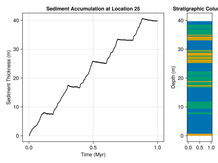

We can clearly see the sediments were removed as their thickness decreases with each regression cycle.