This practical explores how trait evolution is influenced by stratigraphic architectures.
Introduction
Fossils found in a section can provide important insight into evolutionary dynamics over timescales not accessible to direct observations in the presents. The morphological evolution of these fossils allows us to construct stratophenetic series, which are successions of fossils and their traits observed within a stratigraphic section (Dzik 2005). Such fossil time or stratigraphic series allow us to examine how the mode of evolution changes over macroevolutionary timescales, and what the dominant mode of evolution is.
There are multiple “modes of evolution” discussed in the literature, such as stasis, random walk, or Ornstein-Uhlenbeck, which represents convergence to a phenotypic optimum. Each mode reflects an idea of the driving forces of evolution, e.g., the random walk model assumes change in traits is cumulative and random.
Because of the incompleteness of the fossil record, evolutionary biologists tend to be generally skeptical of inferences made from fossil time series, which is most famously reflected in the gradualism vs. punctuated equilibrium debate (Eldredge and Gould 1972). However, it seems that current methods of reconstructing the mode of evolution are surprisingly robust with respect to records with regular gaps (Hohmann et al. 2024).
In this practical, we will build on our understanding of age-depth models and stratigraphic architectures to explore how the stratigraphic record shapes our understanding of morphological evolution along a lineage. Specifically, we will examine when and how stratigraphy can lead to erroneous identification of the mode of evolution.
Coding cheat sheet
Modes of evolution in the time domain
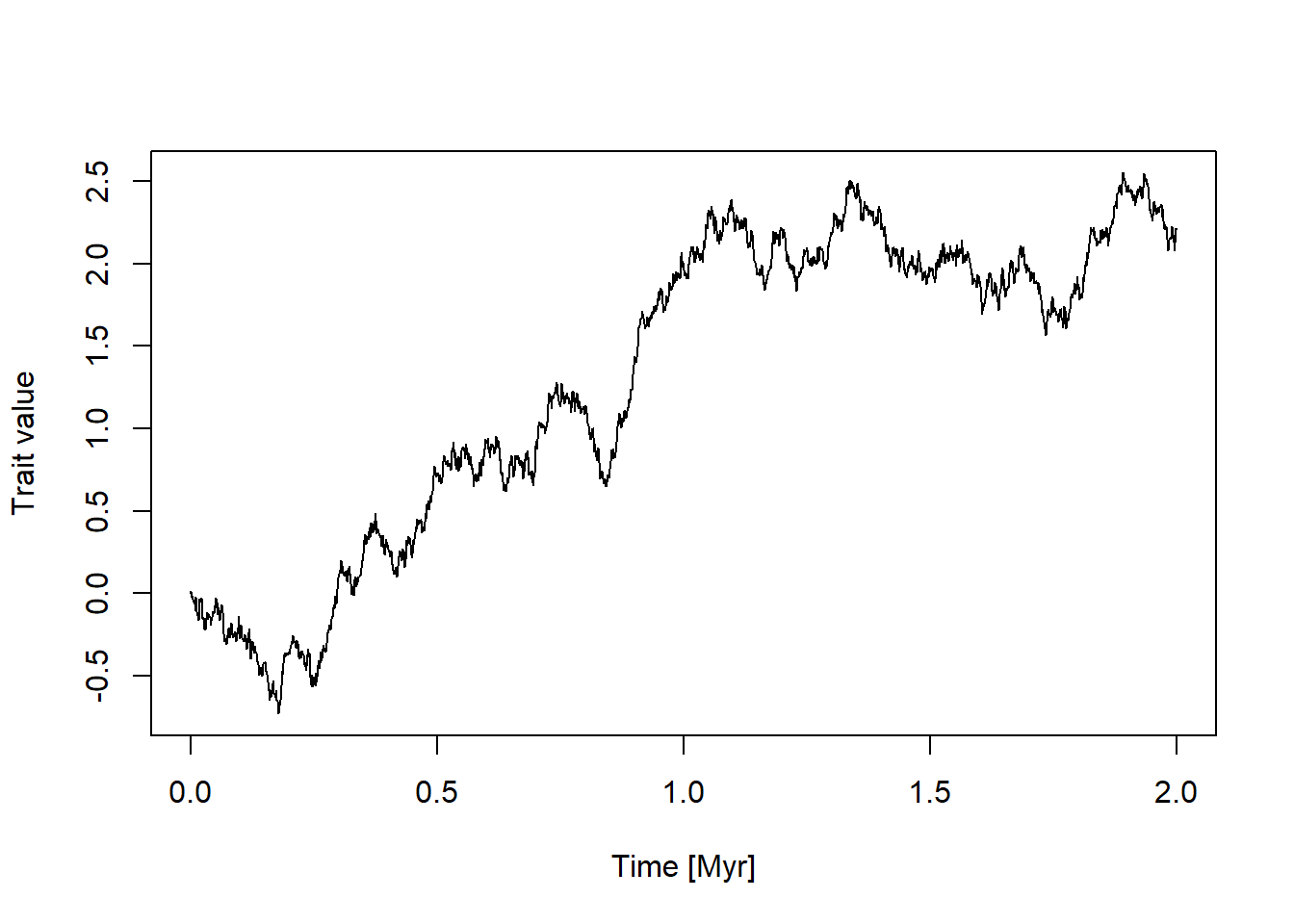
There are three modes of evolution implemented in the StratPal package: stasis, random_walk, and ornstein_uhlenbeck. You can plot them using piping via
library(StratPal)library(admtools)pos ="2km"adm =tp_to_adm(t = scenarioA$t_myr, h = scenarioA$h_m[,pos],T_unit ="Myr",L_unit ="m")temp_res =0.001# temporal resolution in Myrseq(min_time(adm), max_time(adm), by = temp_res) |># time steps where the trait evolution is simulatedrandom_walk(sigma =1, mu =0, y0 =0) |># simulate trait evolutionplot(xlab =paste0("Time [",get_T_unit(adm),"]"), # plotylab ="Trait value",type ="l")
To plot other modes, replace random_walk by one of the other modes (stasis or ornstein_uhlenbeck). If you use stasis, remove the unused arguments - this mode of evolution is simulated using fewer parameters than the others.
Transforming trait evolution into the stratigraphic domain
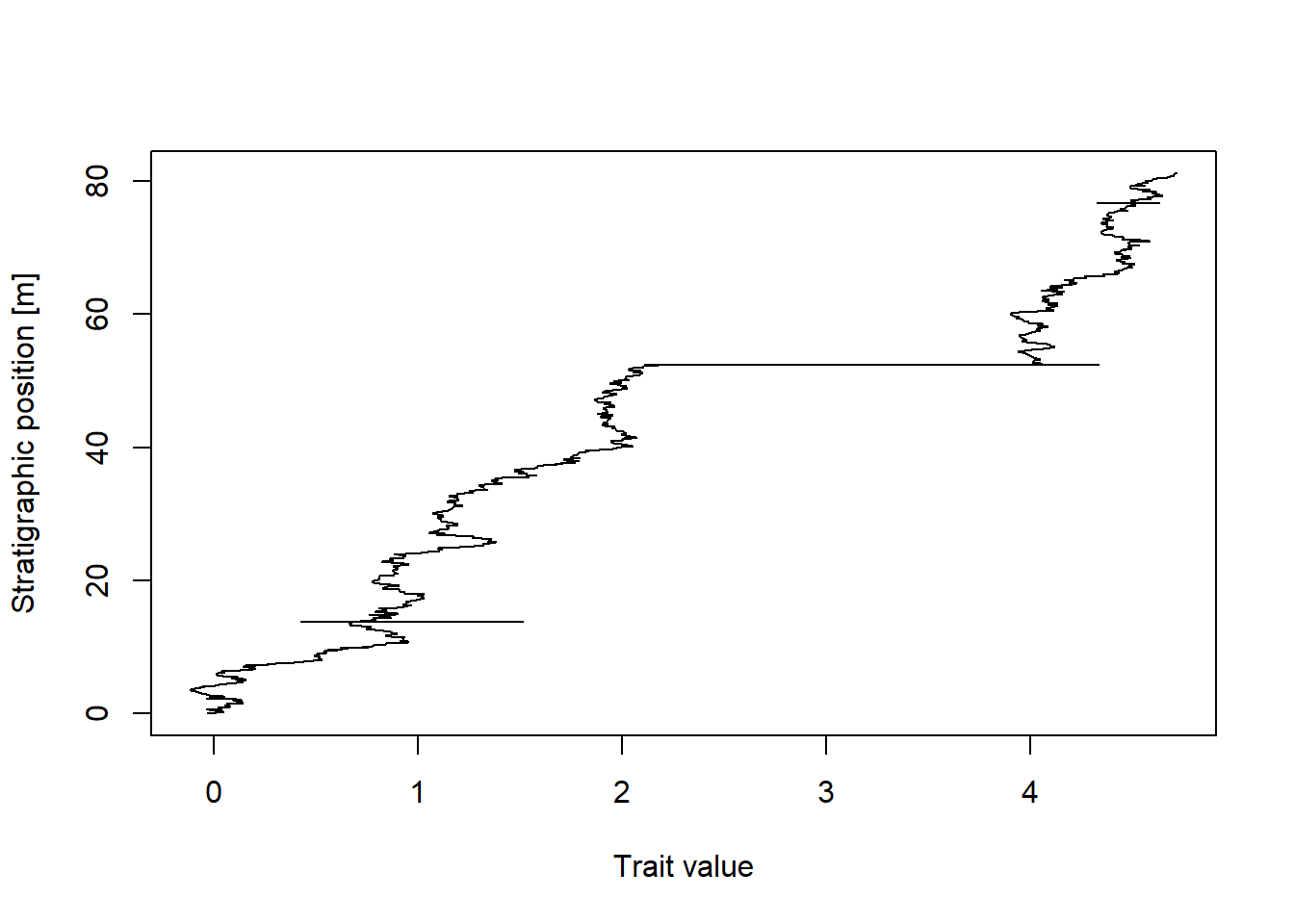
To transform trait evolution into the stratigraphic domain, insert time_to_strat with the age-depth model of your choice into your pipeline:
temp_res =0.001# temporal resolution in Myrseq(min_time(adm), max_time(adm), by = temp_res) |># time steps where the trait evolution is simulatedrandom_walk(sigma =1, mu =3, y0 =0) |># simulate trait evolutiontime_to_strat(adm, destructive =FALSE) |># transform into stratigraphic domainplot(ylab =paste0("Stratigraphic position [",get_L_unit(adm),"]"), # plotxlab ="Trait value",type ="l",orientation ="du")
This will transform your simulations from the time domain into the stratigraphic domain. We use the plotting option orientation = "du" to plot stratigraphic height on the y axis. Use "lr" to plot it on the x axis.
Model selection using the paleoTS package
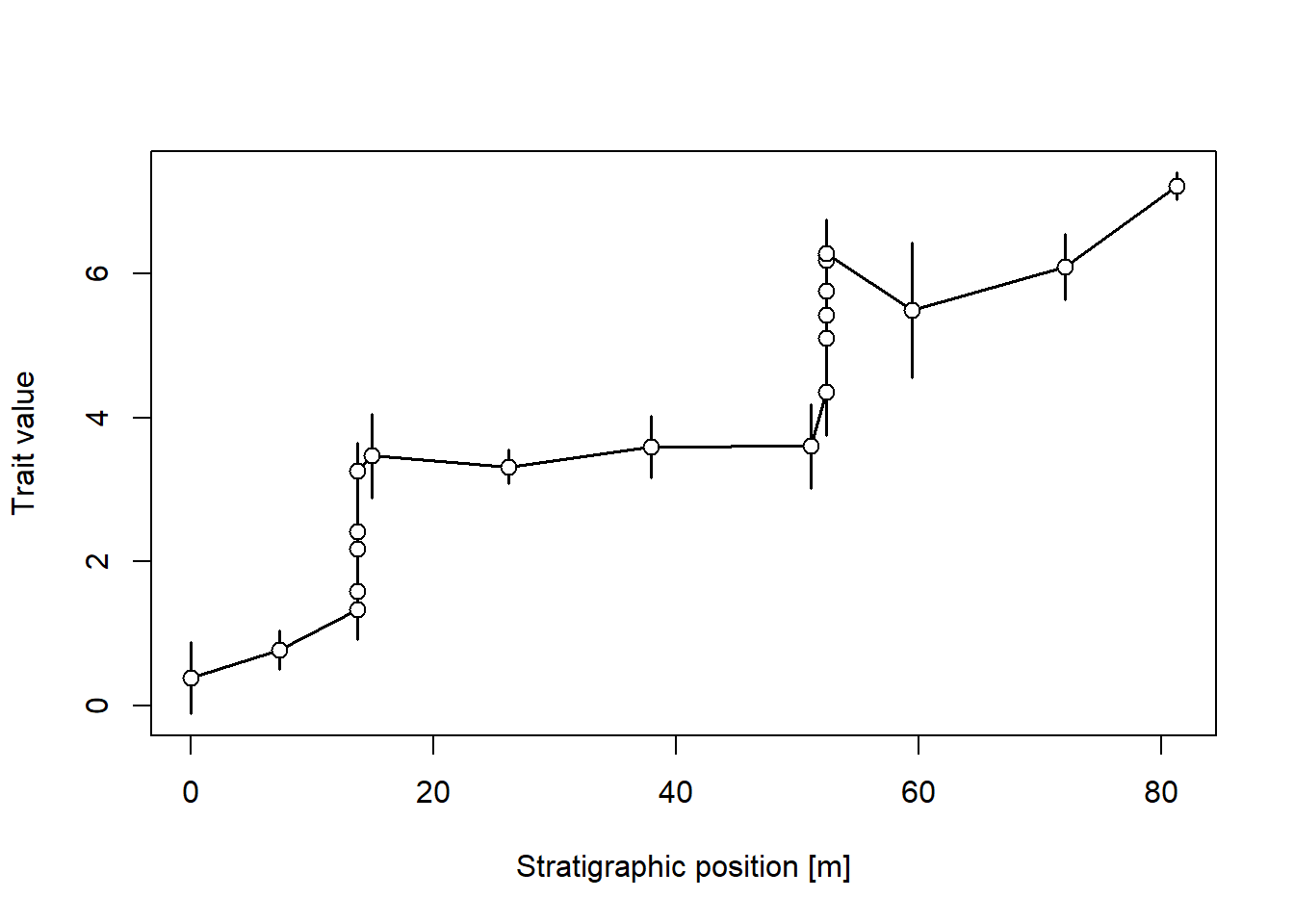
To work with model selection, we need to simulate traits of individuals, not just means of populations as we did above. This is indicated by using the suffix _sl (for “specimen level”) in the simulation.
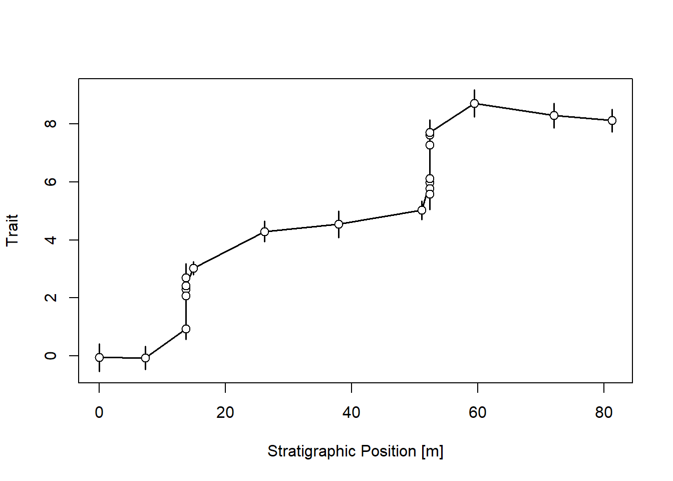
library(paleoTS) # load paleoTS package for model selection & plottingtemp_res =0.1# temporal resolution in Myrseq(min_time(adm), max_time(adm), by = temp_res) |># time steps where the trait evolution is simulatedrandom_walk_sl(sigma =1, mu =3, y0 =0, intrapop_var =1, n_per_sample =5) |># simulate trait evolutiontime_to_strat(adm, destructive =FALSE) |>reduce_to_paleoTS() |># transform into stratigraphic domainplot(xlab =paste0("Stratigraphic position [",get_L_unit(adm),"]"), # plotylab ="Trait value")
We use reduce_to_paleoTS to convert the specimen level simulations from StratPal to the sample level summaries used by paleoTS, see ?reduce_to_paleoTS for details. We can then directly pass the results to the model selection options available in paleoTS (fit3models, fit4models and fit9models, see paleoTS for details):
temp_res =0.1# temporal resolution in Myrintrapop_var =1# trait variance per sampling location/ fossil assemblagen_per_sample =5# number of fossils found per sampling location / fossil assemblageseq(min_time(adm), max_time(adm), by = temp_res) |># time steps where the trait evolution is simulatedrandom_walk_sl(sigma =1, mu =3, y0 =0, intrapop_var = intrapop_var, n_per_sample = n_per_sample) |># simulate trait evolutiontime_to_strat(adm, destructive =FALSE) |>reduce_to_paleoTS() |>fit9models(pool =FALSE)
See the help of the paleoTS package for details on the output and fitSimple to fit more specialized models; more information can be found in (Hunt and G. 2006).
Tasks
You can solve the first two tasks interactively using DarwinCAT.
Task 2.1: Trait evolution in the time domain
Plot the three modes of evolution in the time domain, varying the parameters.
What is their internal variation due to randomness (i.e., how much do results differ if you plot them multiple times)?
What is the biological meaning of the model parameters?
Task 2.2: Stratigraphic effects on trait evolution
Transform the modes of evolution you simulated in the previous step into the stratigraphic domain and plot them.
Which modes are the most/least affected by stratigraphic biases?
Do you see any systematic changes?
Task 2.3: Model selection in the stratigraphic domain
Run model selection on your simulations using the paleoTS package, and compare results from the time and the stratigraphic domain.
Do you see any systematic biases?
Do the results match how you would describe the mode of evolution?
Solutions
You can also explore this topic interactively using DarwinCAT.
Solution Task 2.1: Trait evolution in the time domain
Plot the different modes of evolution in the time domain.
What is their internal variation due to randomness (i.e., how much do results differ if you plot them multiple times)?
What is the biological meaning of the model parameters?
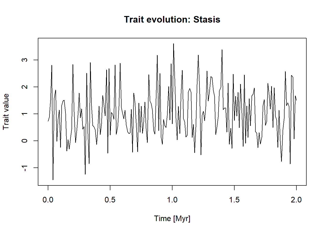
# Stasismin_t =0# beginning observation [Myr]max_t =2# end observation [Myr]t_step =0.01# temporal resolution [Myr]mean =1# model parameter, to modifysd =1# model parameter, to modifyseq(from = min_t, to = max_t, by = t_step) |>stasis(mean = mean, sd = sd) |>plot(type ="l",xlab ="Time [Myr]",ylab ="Trait value",main ="Trait evolution: Stasis")
For stasis, the mean parameter determines the mean trait value, and the sd (standard deviation) parameter determines the spread of trait values. Trait values at individual times are uncorrelated, so if the temporal resolution is increased, trait evolution appears more irregular.
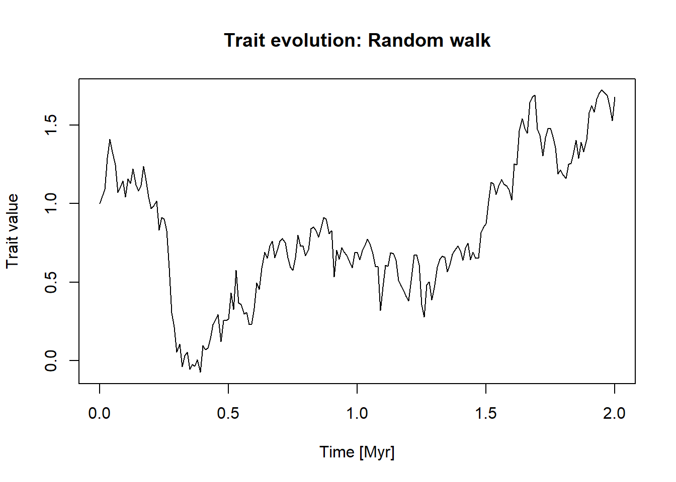
# Random walkmin_t =0# beginning observation [Myr]max_t =2# end observation [Myr]t_step =0.01# temporal resolution [Myr]sigma =1# model parameter, to modifymu =1# model parameter, to modifyy0 =1# model parameter, to modifyseq(from = min_t, to = max_t, by = t_step) |>random_walk(sigma = sigma, mu = mu, y0 = y0) |>plot(type ="l",xlab ="Time [Myr]",ylab ="Trait value",main ="Trait evolution: Random walk")
For the random walk model, the y0 parameter determines the initial trait value. The parameter mu determines the directionality, with positive (negative) values leading to increasing (decreasing) trait values with time. The sigma parameter determines the amount of randomness in the system, with larger values reflecting more randomness. Internal variability is high for larger values of sigma, meaning individual lineages simulated will differ a lot from each other.
Important endmembers are: sigma set to 0, trait evolution is purely deterministic and specified by mu and y0. If mu and y0 are set to 0, trait evolution follows an unbiased random walk model. If sigma is set to 1, the model corresponds to a Brownian motion. For low values of sigma and mu, the random walk can be mistaken for stasis.
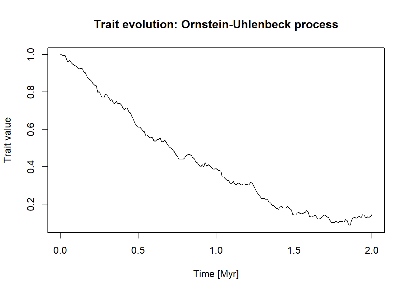
# Ornstein-Uhlenbeckmin_t =0# beginning observation [Myr]max_t =2# end observation [Myr]t_step =0.01# temporal resolution [Myr]theta =1# model parameter, to modifysigma =0.1# model parameter, to modifymu =0# model parameter, to modifyy0 =1# model parameter, to modifyseq(from = min_t, to = max_t, by = t_step) |>ornstein_uhlenbeck(mu = mu, theta = theta, sigma = sigma, y0 = y0) |>plot(type ="l",xlab ="Time [Myr]",ylab ="Trait value",main ="Trait evolution: Ornstein-Uhlenbeck process")
For the Ornstein-Uhlenbeck (OU) model, the parameter y0 represents the initial trait value. The parameter mu determines the long term mean of the process, theta how fast this mean is approached, and sigma how strong the influence of randomness is. This model is used to model convergence from an initial trait value y0 to an optimum mu under pressure of selection theta and random influences sigma.
Internal variation is determined by the sigma parameter, where larger values result in greater variation in simulated trait values.
Important endmembers of the OU model are:
autocorrelated stasis, when y0 = mu (start in the optimum)
directional evolution when the optimum mu is far away from the initial trait value y0, and selection is present
random walk when selection theta is 0
Solution Task 2.2: Stratigraphic effects on trait evolution
Transform the different modes of evolution into the stratigraphic domain and plot them.
Which modes are most/least affected by stratigraphic biases?
Do you see any systematic changes?
Example code for the random walk model is provided. This can be expanded by replacing the random walk by stasis or the Ornstein-Uhlenbeck process.
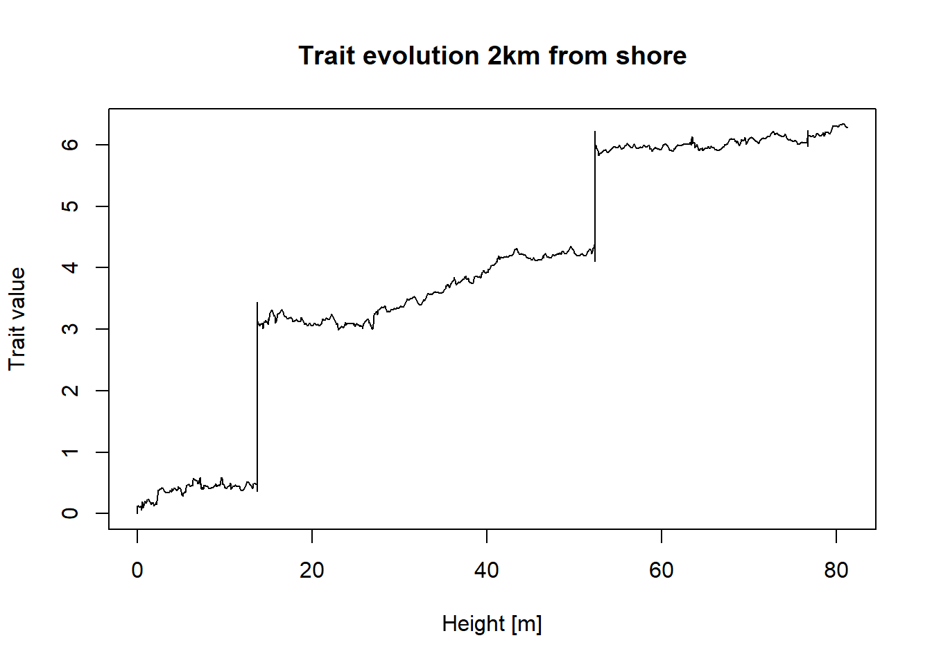
adm_list =list() # storage for age-depth modelsdist =paste(seq(2, 12, by =2), "km", sep ="") # distances from shorefor (pos in dist){ # construct ADMs for all distances adm_list[[pos]] =tp_to_adm(t = scenarioA$t_myr, h = scenarioA$h_m[,pos],T_unit ="Myr",L_unit ="m")}pos ="2km"# position on platformmu =2# model parameterssigma =1# model parametersy0 =0# model paramtersadm = adm_list[[pos]] # select age-depth modelt_step =0.001# temporal resolution [Myr]## plot trait evolution in the stratigraphic domainseq(from =min_time(adm), to =max_time(adm), by = t_step) |>random_walk(sigma = sigma, mu = mu, y0 = y0) |>time_to_strat(adm, destructive =FALSE) |>plot(ylab ="Trait value",type ="l",orientation ="lr",xlab ="Height [m]",main =paste0("Trait evolution ", pos, " from shore") )
Stasis is unaffected by stratigraphic biases. This is because if there is no net change of traits in the time domain, losing parts of the lineage because of hiatuses does not affect the overall pattern.
For the random walk and the Ornstein-Uhlenbeck process, the degree of bias depends on the directionality of evolution. The more the traits change over a hiatus or a condensed interval, the more the stratigraphic expression of trait evolution differs from the one in the time domain. As a result, stratigraphic biases are strongest in the random walk model for large mu, and in the Ornstein-Uhlenbeck model for large differences between y0 and mu.
The effects are strongest if
There are long hiatuses or
There are long intervals of sedimentary condensation.
As a result, stratigraphic biases are driven by maximum hiatus duration on the platform top. This effect is more pronounced the more directional evolution is.
Solution Task 2.3: Model selection in the stratigraphic domain
Run model selection on your simulation using the paleoTS package, and compare results from the time and the stratigraphic domain.
Do you see any systematic biases?
We run model selection both in the stratigraphic and time domain, fitting 9 models to the fossil time series. The example code performs this analysis for simulations under the random walk model, which can be changed out to the stasis or Ornstein-Uhlenbeck model.
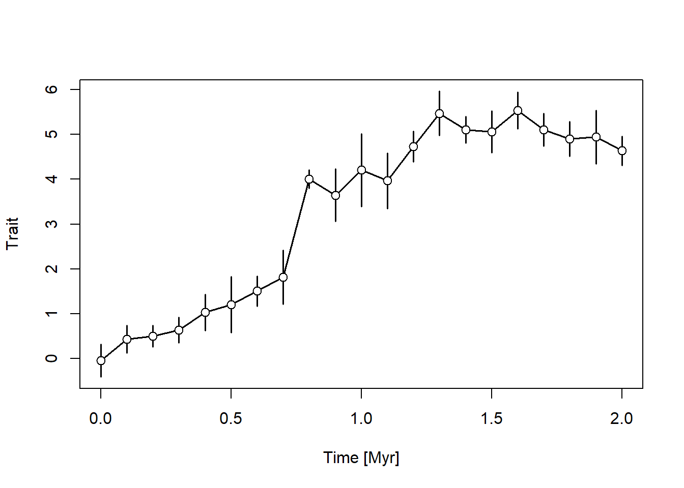
# time domain model selectiontemp_res =0.1# temporal resolution in Myrintrapop_var =1# trait variance per sampling location/ fossil assemblagen_per_sample =5# number of fossils found per sampling location / fossil assemblagetraits_time_domain =seq(min_time(adm), max_time(adm), by = temp_res) |># time steps where the trait evolution is simulatedrandom_walk_sl(sigma =1, mu =3, y0 =0, intrapop_var = intrapop_var, n_per_sample = n_per_sample) |># simulate trait evolutionreduce_to_paleoTS() plot(traits_time_domain, xlab ="Time [Myr]")
Results are sensitive to randomness inherent in the randomness of the simulation, e.g., occasionally a random walk simulation will be identified as stasis even in the abscence of biases. This effect is additionally sensitive to parameters such as sample size and intrapopulation variance (intrapop_var and n_per_sample), reducing the power of the procedure and potentially leading to “analytical stasis”, where low statistical power favors the recovery of stasis (Hannisdal 2006).
Recovery of the correct (meaning, simulated) mode of evolution is better in the time domain, whereas model selection in the stratigraphic domain favors the recognition of punctuated modes of evolution (Hohmann et al. 2024). This effect is strongest in the on the platform top, and disappears on the proximal slope as stratigraphic biases disappear.
As in the visual comparison, stratigraphic effects are strongest the more directional the mode of evolution is, and disappear for stasis.
Stratophenetic time series will thus favor both the recogniton of stasis and punctuated modes of evolution.
References
Dzik, Jerzy. 2005. “THE CHRONOPHYLETIC APPROACH: STRATOPHENETICS FACING AN INCOMPLETE FOSSIL RECORD.”
Eldredge, Niles, and Stephen Jay Gould. 1972. “Punctuated Equilibria: An Alternative to Phyletic Gradualism.” In, edited by Thomas J. M. Schopf, 82115. Freeman Cooper.
Hannisdal, Bjarte. 2006. “Phenotypic Evolution in the Fossil Record: Numerical Experiments.”The Journal of Geology 114 (2): 133–53. https://doi.org/10.1086/499569.
Hohmann, Niklas, Joël R. Koelewijn, Peter Burgess, and Emilia Jarochowska. 2024. “Identification of the Mode of Evolution in Incomplete Carbonate Successions.”BMC Ecology and Evolution 24 (1): 113. https://doi.org/10.1186/s12862-024-02287-2.
Hunt, and G. 2006. “Fitting and Comparing Models of Phyletic Evolution: Random Walks and Beyond.”Paleobiology 32 (4): –23. https://doi.org/10.1666/05070.1.