Models niches by removing events (fossil occurrences) or specimens when they are outside of their niche. For event type data, this is done using the function thin, for pre_paleoTS this is done by applying the function prob_remove on the specimens. For fossils objects produced by the FossilSim package, fossil observations are removed according to the specified niche
Combines the functions niche_def and gc ("gradient change") to determine how the taxons' collection probability changes with time/position. This is done by composing niche_def and gc. The result is then used to remove events/specimens in x.
Arguments
- x
events type data, e.g. vector of times/ages of fossil occurrences or their stratigraphic position, or a
pre_paleoTSobject (e.g. produced bystasis_sl), or afossilsobject produced by theFossilSimpackage.- niche_def
function, specifying the niche along a gradient. Should return 0 when taxon is outside of niche, and 1 when inside niche. Values between 0 and 1 are interpreted as collection probabilities. Must be vectorized, meaning if given a vector, it must return a vector of equal length.
- gc
function, stands for "gradient change". Specifies how the gradient changes, e.g. with time. Must be vectorized, meaning if given a vector, it must return a vector of equal length.
Value
for a numeric vector input, returns a numeric vector, timing/location of events (e.g. fossil ages/locations) preserved after the niche model is applied. For a pre_paleoTS object as input, returns a pre_paleoTS object with specimens removed according to the niche model. For a fossils object, returns a fossils object with some occurrences removed according to the niche definition
See also
snd_niche()andbounded_niche()for template niche models,discrete_niche()anddiscrete_gradient()to construct niches from discrete categories,trivial_niche()to model organisms without niche specificationsvignette("advanced_functionality)for how to create user-defined niche modelsapply_taphonomy()to model taphonomic effects based on a similar principlethin()andprob_remove()for the underlying mathematical procedures
Examples
### example for event type data
## setup
# using water depth as gradient
t = scenarioA$t_myr
wd = scenarioA$wd_m[,"8km"]
gc = approxfun(t, wd)
plot(t, gc(t), type = "l", xlab = "Time", ylab = "water depth [m]",
main = "gradient change with time")
 # define niche
# preferred wd 10 m, tolerant to intermediate wd changes (standard deviation 10 m), non-terrestrial
niche_def = snd_niche(opt = 10, tol = 10, cutoff_val = 0)
plot(seq(-1, 50, by = 0.5), niche_def(seq(-1, 50, by = 0.5)), type = "l",
xlab = "water depth", ylab = "collection probability", main = "Niche def")
# define niche
# preferred wd 10 m, tolerant to intermediate wd changes (standard deviation 10 m), non-terrestrial
niche_def = snd_niche(opt = 10, tol = 10, cutoff_val = 0)
plot(seq(-1, 50, by = 0.5), niche_def(seq(-1, 50, by = 0.5)), type = "l",
xlab = "water depth", ylab = "collection probability", main = "Niche def")
 # niche pref with time
plot(t, niche_def(gc(t)), type = "l", xlab = "time",
ylab = "collection probability", main = "collection probability with time")
# niche pref with time
plot(t, niche_def(gc(t)), type = "l", xlab = "time",
ylab = "collection probability", main = "collection probability with time")
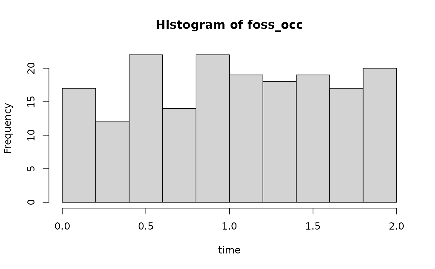
 ## simulate fossil occurrences
foss_occ = p3(rate = 100, from = 0, to = max(t))
# foss occ without niche pref
hist(foss_occ, xlab = "time")
## simulate fossil occurrences
foss_occ = p3(rate = 100, from = 0, to = max(t))
# foss occ without niche pref
hist(foss_occ, xlab = "time")
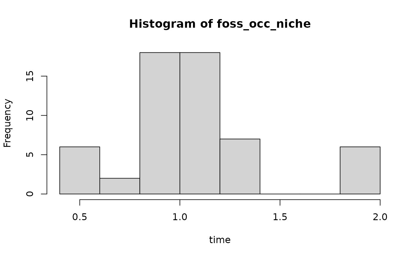
 foss_occ_niche = apply_niche(foss_occ, niche_def, gc)
# fossil occurrences with niche preference
hist(foss_occ_niche, xlab = "time")
foss_occ_niche = apply_niche(foss_occ, niche_def, gc)
# fossil occurrences with niche preference
hist(foss_occ_niche, xlab = "time")
 # see also
#vignette("event_data")
# for a detailed example on niche modeling for event type data
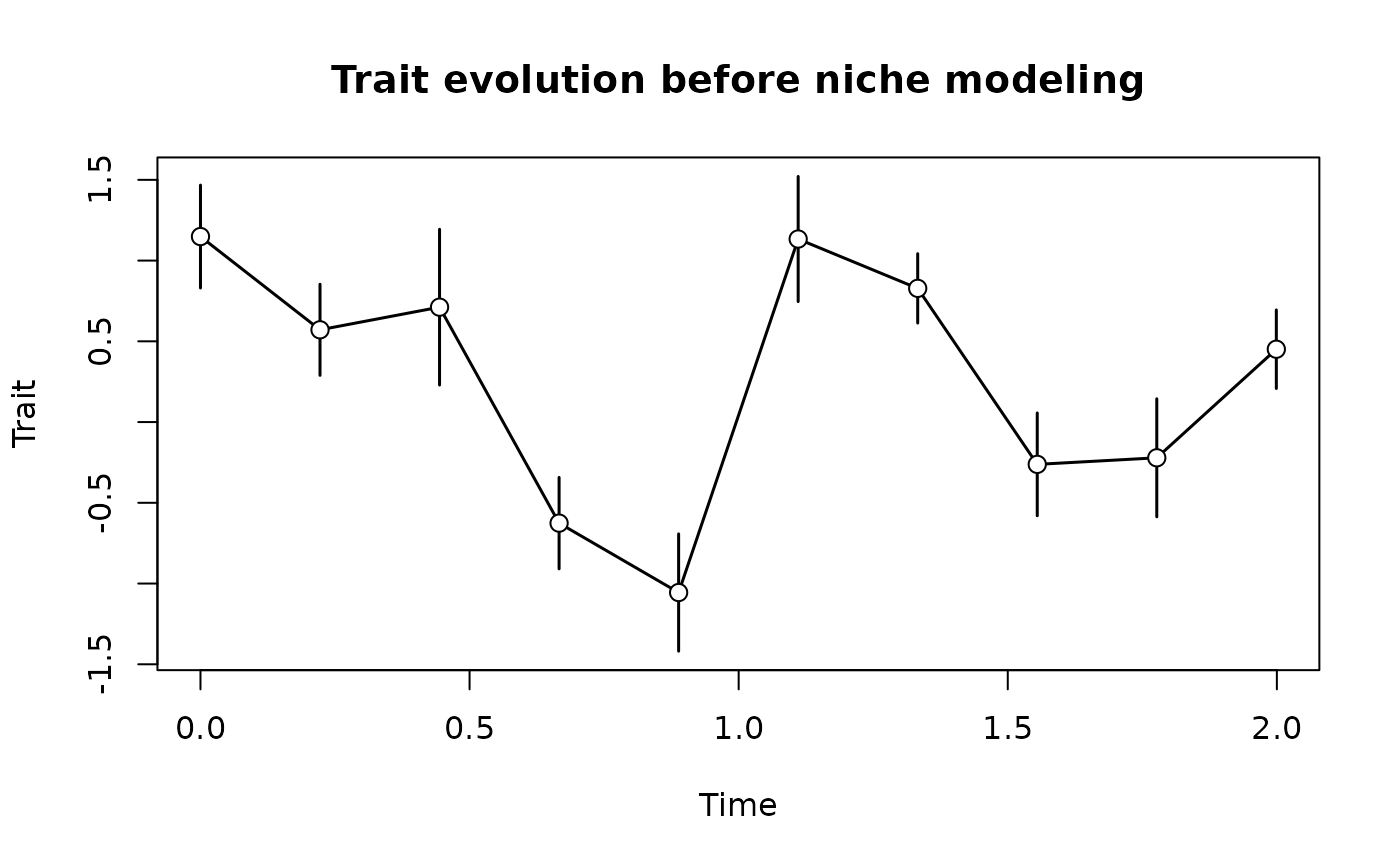
### example for pre_paleoTS objects
# we reuse the niche definition and gradient change from above!
x = stasis_sl(seq(0, max(t), length.out = 10))
plot(reduce_to_paleoTS(x), main = "Trait evolution before niche modeling")
# see also
#vignette("event_data")
# for a detailed example on niche modeling for event type data
### example for pre_paleoTS objects
# we reuse the niche definition and gradient change from above!
x = stasis_sl(seq(0, max(t), length.out = 10))
plot(reduce_to_paleoTS(x), main = "Trait evolution before niche modeling")
 y = apply_niche(x, niche_def, gc)
plot(reduce_to_paleoTS(y), main = "Trait evolution after niche modeling",
ylim = c(-2, 2))
y = apply_niche(x, niche_def, gc)
plot(reduce_to_paleoTS(y), main = "Trait evolution after niche modeling",
ylim = c(-2, 2))
 # note that there are fewer sampling sites
# bc the taxon does not appear everywhere
# and there are fewer specimens per sampling site
### example for fossils objects
# we reuse the niche definition and gradient change from above
# simulate tree
tree = ape::rlineage(birth = 2, death = 0, Tmax = 2)
# create fossils object
f = FossilSim::sim.fossils.poisson(rate = 2, tree = tree)
# plot fossils along tree before niche model is applied
FossilSim:::plot.fossils(f, tree = tree)
# note that there are fewer sampling sites
# bc the taxon does not appear everywhere
# and there are fewer specimens per sampling site
### example for fossils objects
# we reuse the niche definition and gradient change from above
# simulate tree
tree = ape::rlineage(birth = 2, death = 0, Tmax = 2)
# create fossils object
f = FossilSim::sim.fossils.poisson(rate = 2, tree = tree)
# plot fossils along tree before niche model is applied
FossilSim:::plot.fossils(f, tree = tree)
 # introduce niche model
f_mod = f |>
admtools::rev_dir(ref = max(t)) |> # reverse direction bc FossilSim uses age not time
apply_niche(niche_def, gc) |>
admtools::rev_dir(ref = max(t))
# plot fossils along tree after introduction of niche model
FossilSim:::plot.fossils(f_mod, tree = tree)
# introduce niche model
f_mod = f |>
admtools::rev_dir(ref = max(t)) |> # reverse direction bc FossilSim uses age not time
apply_niche(niche_def, gc) |>
admtools::rev_dir(ref = max(t))
# plot fossils along tree after introduction of niche model
FossilSim:::plot.fossils(f_mod, tree = tree)
 # note how only fossils in the interval where environmental conditions are suitable are preserved
# note that FossilSim uses age before the present, which is why we use admtools::rev_dir
# note how only fossils in the interval where environmental conditions are suitable are preserved
# note that FossilSim uses age before the present, which is why we use admtools::rev_dir