simulate ornstein-uhlenbeck (OU) process

Simulates an Ornstein-Uhlenbeck process using the Euler-Maruyama method. The process is simulated on a scale of 0.25 * min(diff(t)) and then interpolated to the values of t.

Usage

ornstein_uhlenbeck(t, mu = 0, theta = 1, sigma = 1, y0 = 0)

Arguments

t

times at which the process is simulated. Can be heterodistant

mu

scalar, long term mean

theta

scalar, mean reversion speed

sigma

positive scalar, strength of randomness

y0

scalar, initial value (value of process at the first entry of t)

Value

A list with two elements: t and y. t is a duplicate of the input t, y are the values of the OU process at these times. Output list is of S3 class timelist (inherits from list) and can thus be plotted directly using plot, see ?admtools::plot.timelist

Examples

library("admtools") # required for plotting of results
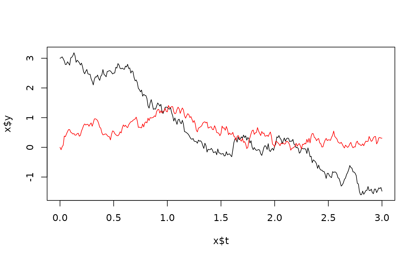
t = seq(0, 3, by = 0.01)
l = ornstein_uhlenbeck(t, y0 = 3) # start away from optimum (mu)
plot(l, type = "l")
l2 = ornstein_uhlenbeck(t, y0 = 0) # start in optimum
lines(l2$t, l2$y, col = "red")