Estimating Age-Depth Models from Sedimentation Rates

Introduction

This vignette explains how to estimate age-depth models (ADMs) from sedimentation rates and tie points using the function sedrate_to_multiadm

Inputs

The sedrate_to_multiadm function estimates age-depth models from sedimentation rates and position and timing of tie points. It takes the following inputs that encode user knowledge:

h_tp : a function encoding stratigraphic positions of tie points
t_tp : a function encoding times of the tie points
sed_rate_gen: a function encoding how sedimentation rates change with stratigraphic positions. This information can for example be derived from cyclostratigraphic analyses.

In addition, it takes the following inputs that specify the estimation procedure:

h : vector of heights where the ADM is determined
no_of_rep: integer, number of runs

Additional parameters that determine the numeric behavior of the integration method used are subdivisions and stop.on.error. The parameters T_unit and L_unit can be used to associate time and length units with the generated age-depth model.

Example

We construct an age depth model for a section of 10 m thickness where upper and lower bounds on sedimentation rates are available. This is a simplified example, details on how arbitrary sedimentation rates can be encoded can be found below.

Data

We start by defining the section as well as lower and upper bounds on sedimentation rates

h_min = 2 # lower boundary of the section
h_max = 10 # upper boundary of the section
T_unit = "Myr"
L_unit = "m"

We want to know the age-depth model every 10 cm, so we define

h = seq(h_min, h_max, by = 0.1)

Tie points

We assume there is one tie point in the section at 5 m height, and its mean age is 66 years with a standard deviation of 0.25 Myr

h1 = 5
mean_age = -66
sd = 0.25

Then the tie point timing is given by

t_tp = tp_time_norm(mean = mean_age, sd = sd)

and the tie point height is given by

h_tp = tp_height_det(heights = h1)

Every time t_tp is evaluated, it returns one possible time of the tie points. Similarly, every time h_tp is evaluated, it returns the stratigraphic position of the tie point (which is deterministic in this case):

h_tp()
#> [1] 5
t_tp()
#> [1] -66.35001

Sedimentation rates

We assume the following upper and lower limits for sedimentation rates:

sedrate_max_y = c(2,5,8,5)
sedrate_max_x = c(1,4,6,10)
sedrate_min_y = c(1,1,7,0.5)
sedrate_min_x = sedrate_max_x

Here, sedrate_max_y[i] is the upper limit on sedimentation rate at sedrate_max_x[i] (mutatis mutandis for sedrate_min). Between these points, we assume linear interpolation. This is done by the function sed_rate_gen_from_bounds:

sedrate = sed_rate_gen_from_bounds(h_l = sedrate_min_x,
                                   s_l = sedrate_min_y,
                                   h_u = sedrate_max_x,
                                   s_u = sedrate_max_y,
                                   rate = 1)

Because the sedimentation rates are uncertain, functions returned by sedrate will differ each time the function is evaluated. As an example, we plot three different sample paths (realizations) of the sedimentation rate through the section:

plot(NULL,
     xlim = range(h),
     ylim = c(0, max(c(sedrate_max_y))),
     xlab = "Height [m]",
     ylab = "Sedimentation Rate [m/Myr]")
no_sedrates = 3
cols = c("red", "blue", "black")
for (i in seq_len(no_sedrates)){
  sedrate_sample = sedrate()
  lines(h, sedrate_sample(h), lwd = 3, col = cols[i])
}

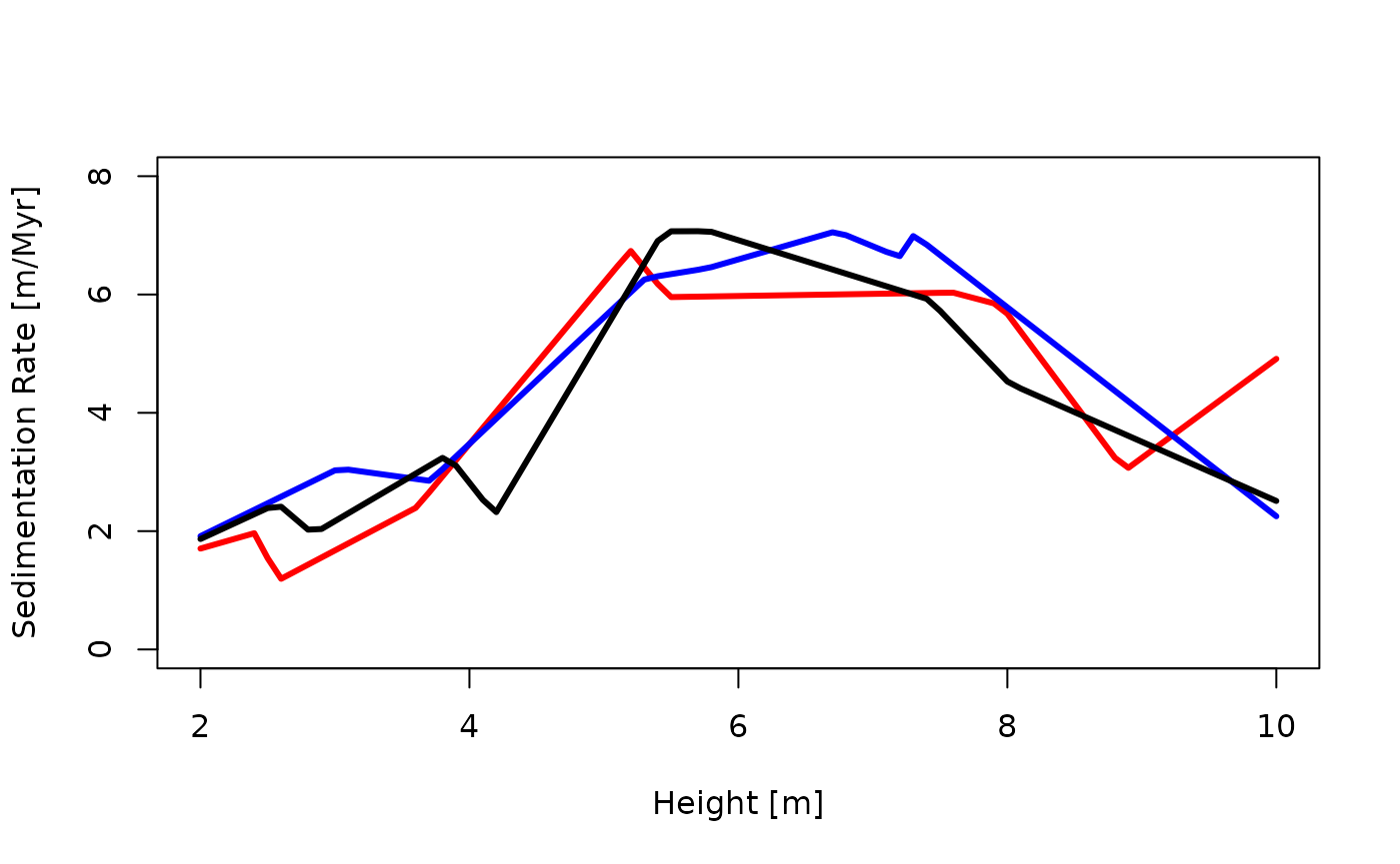
These sedimentation rates assume sedimentation rates are drawn from a uniform distribution between the upper and lower limits of sedimentation rate provided by the user. This is done at random locations determined according to a Poisson point process with rate rate.

Estimate age depth model

With tie points and sedimentation rates specified, we can now estimate the age depth model using

my_adm = sedrate_to_multiadm(h_tp = h_tp,
                             t_tp = t_tp,
                             sed_rate_gen = sedrate,
                             h = h,
                             T_unit = T_unit,
                             L_unit = L_unit)

The age-depth model can be plotted using

plot(my_adm)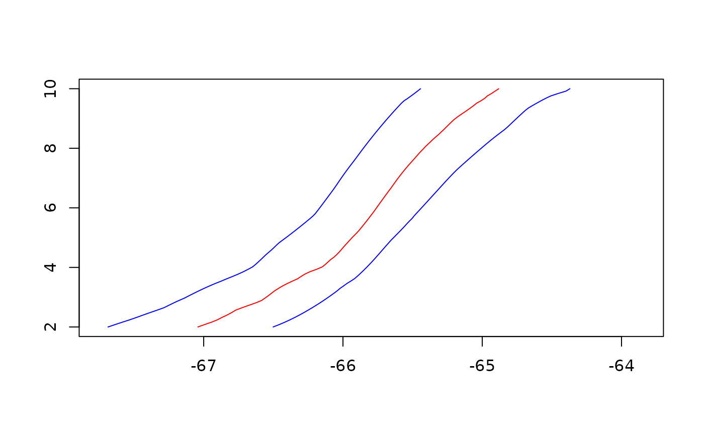

You can extract mean, median, and quantile age-depth models using mean_adm, median_adm and quantile_adm:

mean_adm = mean_adm(my_adm, h)
plot(mean_adm)

Coding tie points

Background

Times and heights of tie points are coded via the functions t_tp (timing) and h_tp (height) that take no inputs. They serve as wrappers around user-defined procedures that reflect uncertainties around tie points. Every time t_tp and h_tp are evaluated, they return possible values for the tie points. Conceptually, both t_tpand h_tp are user implemented random number generators that draw from the distributions of tie points. Writing these functions requires some effort, but it allows the user to hand over arbitrarily complex uncertainties of the tie points to the sedrate_to_multiadm function.

Wrappers

Multiple wrappers are available to simplify coding tie points:

tp_height_det for specifying deterministic stratigraphic heights
tp_time_det for specifying deterministic time points
tp_time_floating_scale to encode time tie points for floating time scale
tp_time_norm for normally distributed tie points in time

Manually coding tie points

Both t_tp and h_tp must return strictly ordered numeric vectors of times/heights. This means that it is the users responsibility to avoid inversions of times/heights.

As an example, I assume the stratigraphic positions of the tie points are known without uncertainty, and are at 10 and 20 m stratigraphic height.

h_min = 10 # stratigraphic height of lower tie point [m]
h_max = 20 # stratigraphic height of upper tie point [m]

h_tp is then implemented as follows:

h_tp = function(){
  return(c(h_min, h_max))
}

When evaluated, this function returns the stratigraphic positions of the tie points:

h_tp()
#> [1] 10 20

Note that the h_tp defined here is a synonym for h_tp = tp_height_det(c(h_min, h_max)).

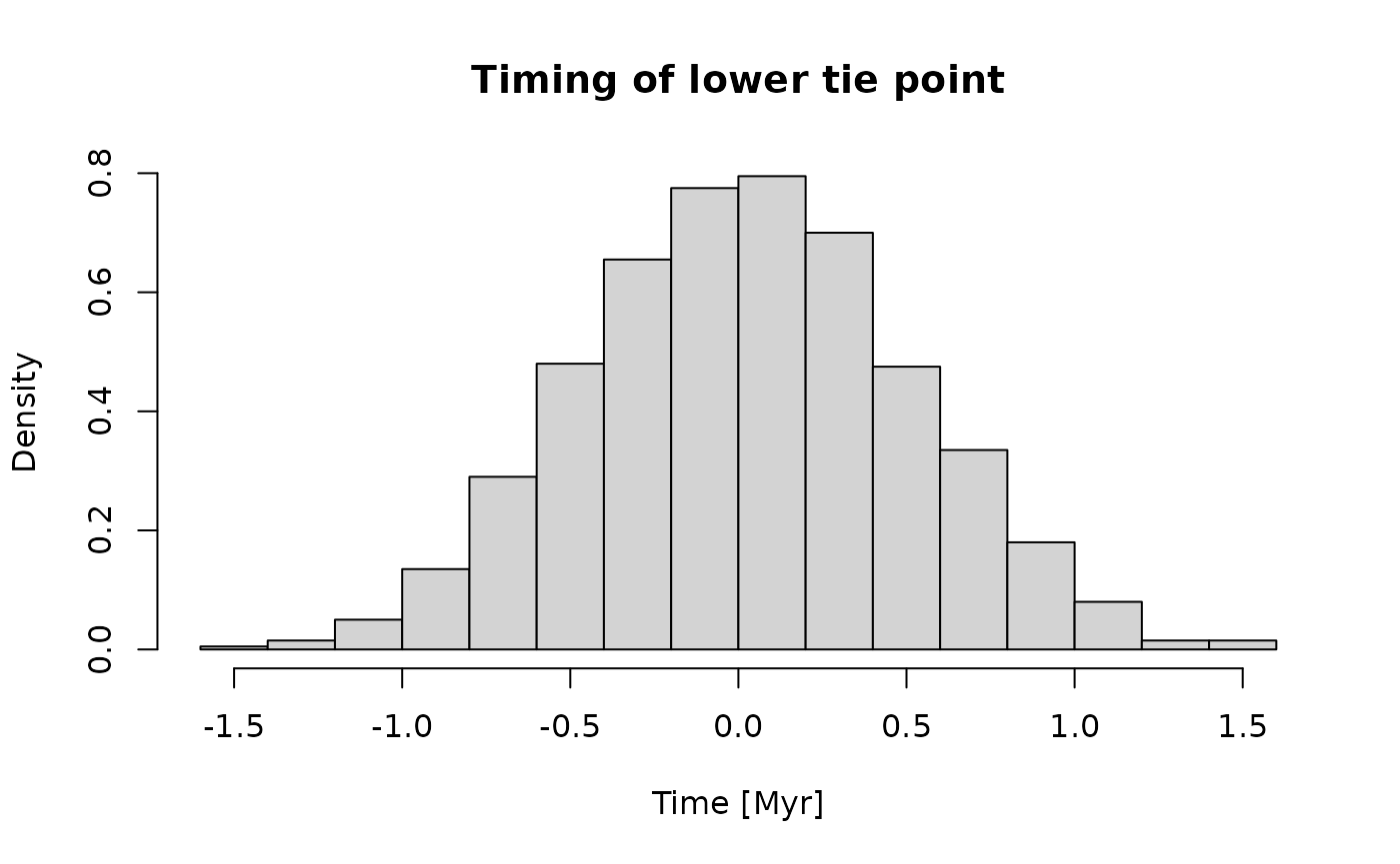
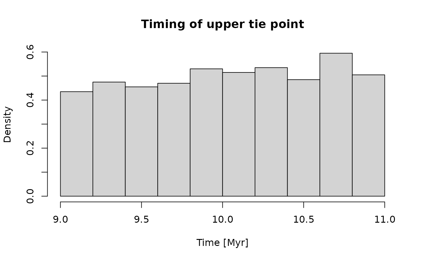
For a more complex example, I assume that the timing of the first tie point follows a normal distribution with mean 0 and standard deviation 0.5. For the second tie point, only maximum and minimum time is available. Due to the lack of information, I assume a uniform distribution between the minimum (9) and the maximum (11). This is implemented as follows in t_tp:

t_tp = function() {
  repeat{ 
    # timing first tie point
    t1 = rnorm(n = 1, mean = 0, sd = 0.5)
    # timing second tie point
    t2 = runif(n = 1, min = 9, max = 11)
    if (t1 < t2){ # if order is correct, return values
        return(c(t1, t2))
    }
  }
}

t_tp() # evaluating the function returns a random pair of times drawn from the specified distribution
#> [1]  0.2729596 10.6250840

Using Myr as time unit, the distribution of times for the tie points is as follows:

Coding sedimentation rates

Background

Mathematically, sedimentation rates are assumed to be stochastic processes. With each iteration of the estimation procedure, a sample path is generated from the stochastic processes. This sample path reflects one possible change of sedimentation rate in the section, given our uncertainties about it.

Computationally, this is implemented using function factories, which are functions that return functions. A function factory defines a stochastic process, and each function $f$ generated by a function factory is a sample path. In turn, $f(x)$ returns the value of the sample path at $x$ .

Here, function factories are used as complex random number generators: Instead of returning one or multiple random numbers, they return a random function.

Wrappers

Available wrappers to define sedimentation rates are

sed_rate_gen_from_bounds : generate sed. rate from upper and lower bounds on the sedimentation rate (see above)
sed_rate_from_matrix: specify sedimentation rate based on matrix, to be used in conjunction with get_data_from_eTimeOpt. This allows to have sedimentation rates change both at deterministic and randomized heights, see ?sed_rate_from_matrix for details.

Manually coding sedimentation rates

Sedimentation rates must be coded as function factories, i.e., functions that return functions. They must be able to take vector inputs and return a vector of the same length as output, and always return strictly positive values.

As example, I use a simple sedimentation rate model, where only upper and lower bounds on sedimentation rates in the section are known. Between these limits, I assume a uniform distribution.

h_min = 10
h_max = 90
# limits on sed. rates 
lower_limit = c(0.1,2,0.1,10) 
upper_limit = c(0.2,3,2,12)  
# strat intervals where sed rates are defined 
s = c(h_min, 30,65, 80, h_max)

Based on these parameters, the sedimentation rate function factory is defined as follows:

# define function factory 
sed_rate_fun = function(){   
  # draw sed rates from uniform distribution  
  aa = runif(n = length(lower_limit), min = lower_limit, max = upper_limit)   
  # define sed rate "realization" based on samples from uniform distribution 
  sed_rate_fun = approxfun(x = s, 
                           y = c(aa, aa[length(aa)]), 
                           method = "constant", 
                           rule = 2,  
                          f = 1) 
  return(sed_rate_fun)
}

Note that the inner function is a function of one variable (height), while the outer function takes no arguments - it simply returns the inner function. To visualize this, let’s plot three sedimentation rates generated by the “sedimentation rate function factory” sed_rate_fun:

plot(NULL,
     xlim = c(h_min, h_max),
     ylim = c(0, max(upper_limit)),
     xlab = "Stratigraphic Height [m]",
     ylab = "Sedimentation Rate")

no_of_sedrates = 3 # no. of sed rates displayed
h = seq(h_min,h_max, by = 0.1) # strat. positions where sed rates are plotted
cols = c("red", "blue", "black")
for (i in seq_len(no_of_sedrates)){
  # generate sed rate from the factory
  sed_rate_sample = sed_rate_fun()
  
  # plot sed rate in the section
  lines(h, sed_rate_sample(h), col = cols[i])
}

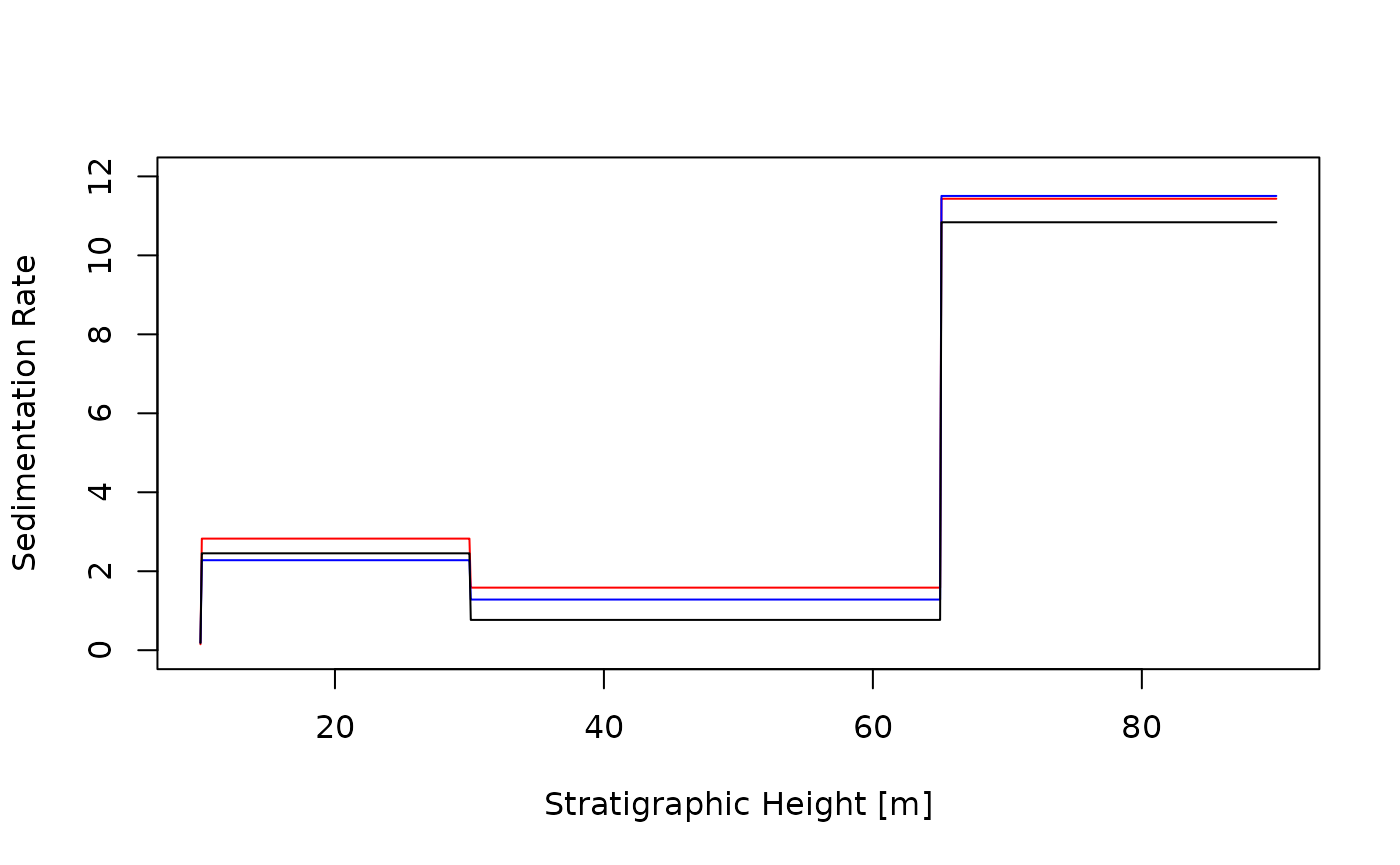
All sedimentation rates generated by sed_rate_fun will be different, because they are determined by random numbers.

Further information

For information on estimating age-depth models from tracer contents of rocks and sediments, see

vignette("adm_from_trace_cont")

For details on plotting ADMs see

vignette("adm_plotting)

For an overview of the structure of the admtools package and the classes used therein see

vignette("admtools_doc")

For an overview over all available vignettes for the admtools package use

browseVignettes(package = "admtools")

Niklas Hohmann

Introduction

Inputs

Example

Data

Tie points

Sedimentation rates

Estimate age depth model

Coding tie points

Background

Wrappers

Manually coding tie points

Coding sedimentation rates

Background

Wrappers

Manually coding sedimentation rates

Further information