admtools: Getting Started

Introduction

This vignette is an introduction to the admtools package.

Installation

From GitHub

From CRAN

To install the package from CRAN, run

install.packages("admtools")

To install the package from GitHub, first install the remotes package:

install.packages("remotes")

Then run

remotes::install_github(repo = "MindTheGap-ERC/admtools",
                        build_vignettes = TRUE,
                        ref = "HEAD",
                        dependencies = TRUE)

to install the latest stable version.

Loading the package

Load the package using

library(admtools)

This makes all functions in the package available.

Getting help

Use

help(package = "admtools")

to get an overview of the available help pages of the package, and

?admtools

to view a simple help page for the package.

Vignettes are a long form of package documentation that provide more detailed examples. To list the available vignettes, use

browseVignettes(package = "admtools") # opens in Browser
#or
vignette(package = "admtools")

The adm and multiadm classes

The admtools package defines three main classes: adm, sac and multiadm. The class adm represent a single age-depth model, from which information can be extracted (e.g. completeness, number of hiatuses, etc.) and that can be used to transform data between the stratigraphic domain and time domain. The multiamd class is a list of adm objects. multiadm objects are used to represent uncertainties of age-depth models. Objects of type sac are sediment accumulation curves that can contain information on erosion, and can be turned into age-depth models.

Conventions

In contrast to its name, the admtools package currently deals with time and height instead of age and depth. In this sense, the age-depth models are time-height models. Both time and height can be negative values. To handle ages, use time before the present. To handle depths, use height below a point of reference (e.g., the sediment surface).

Example

This example explains the construction and application of adm objects. As example data we use outputs from CarboCAT Lite, a model of carbonate platform growth (Burgess 2013, 2023). This data is automatically loaded in the background by the package. To get some info of the data use

?CarboCATLite_data

This data is identical to scenario A from Hohmann et al. (2024) as published in Hohmann et al. (2023). See therein for details on the simulation, reproducibility, and a chronostratigraphic chart and a figure showing a transect through the carbonate platform.

Defining age-depth models

The standard constructor for age-depth models is tp_to_adm (“tie point to age-depth model”). It returns an objecto of class adm. This object combines information of stratigraphic heights and times and erosive interval. It allows to transform data between the stratigraphic and the time domain, and identify which data is destroyed due to hiatuses.

As example, I use the timing and stratigraphic positions of tie points taken from CarboCAT Lite to construct an age-depth model, and use the option to directly associate length and time units with it.

# see ?tp_to_adm for detailed documentation
my_adm = tp_to_adm(t = CarboCATLite_data$time_myr,
                  h = CarboCATLite_data$height_2_km_offshore_m,
                  L_unit = "m",
                  T_unit = "Myr")

This age-depth model represents the relationship between elapsed model time and accumulated sediment 2 km offshore in a synthetic carbonate platform.

Representation

Typing the name my_adm in the console will only tell that the generated variable is an age-depth model

my_adm
#> age-depth model

To get a quick overview of the properties of my_adm, use summary:

summary(my_adm)
#> age-depth model 
#> Total duration: 2 Myr
#> Total thickness: 146.0621 m
#> Stratigraphic completeness: 32.65 % 
#> 10 hiatus(es)

If you want to inspect the insides of the object, use str:

str(my_adm)
#> List of 5
#>  $ t     : num [1:2001] 0 0.001 0.002 0.003 0.004 0.005 0.006 0.007 0.008 0.009 ...
#>  $ h     : num [1:2001] 0 0 0.609 1.095 1.722 ...
#>  $ destr : logi [1:2000] TRUE FALSE FALSE FALSE FALSE FALSE ...
#>  $ T_unit: chr "Myr"
#>  $ L_unit: chr "m"
#>  - attr(*, "class")= chr "adm"

You can manually manipulate the fields of the adm object by treating it like a list. I do not recommend doing so, as it might result in unexpected downstream behavior. If you want to extract tie points use get_L_tp and get_T_tp.

You can plot adm objects via the standard plot function. Here, I use the option to highlight hiatuses in red, and increase the linw width of the conservative ( = non-destructive) intervals.

# see ?plot.adm for plotting options for adm objects
plot(my_adm,
     col_destr = "red",
     lwd_acc = 2)
T_axis_lab() # plot time axis label, see ?T_axis_lab for details
L_axis_lab() # plot height axis label, see ?L_axis_lab for details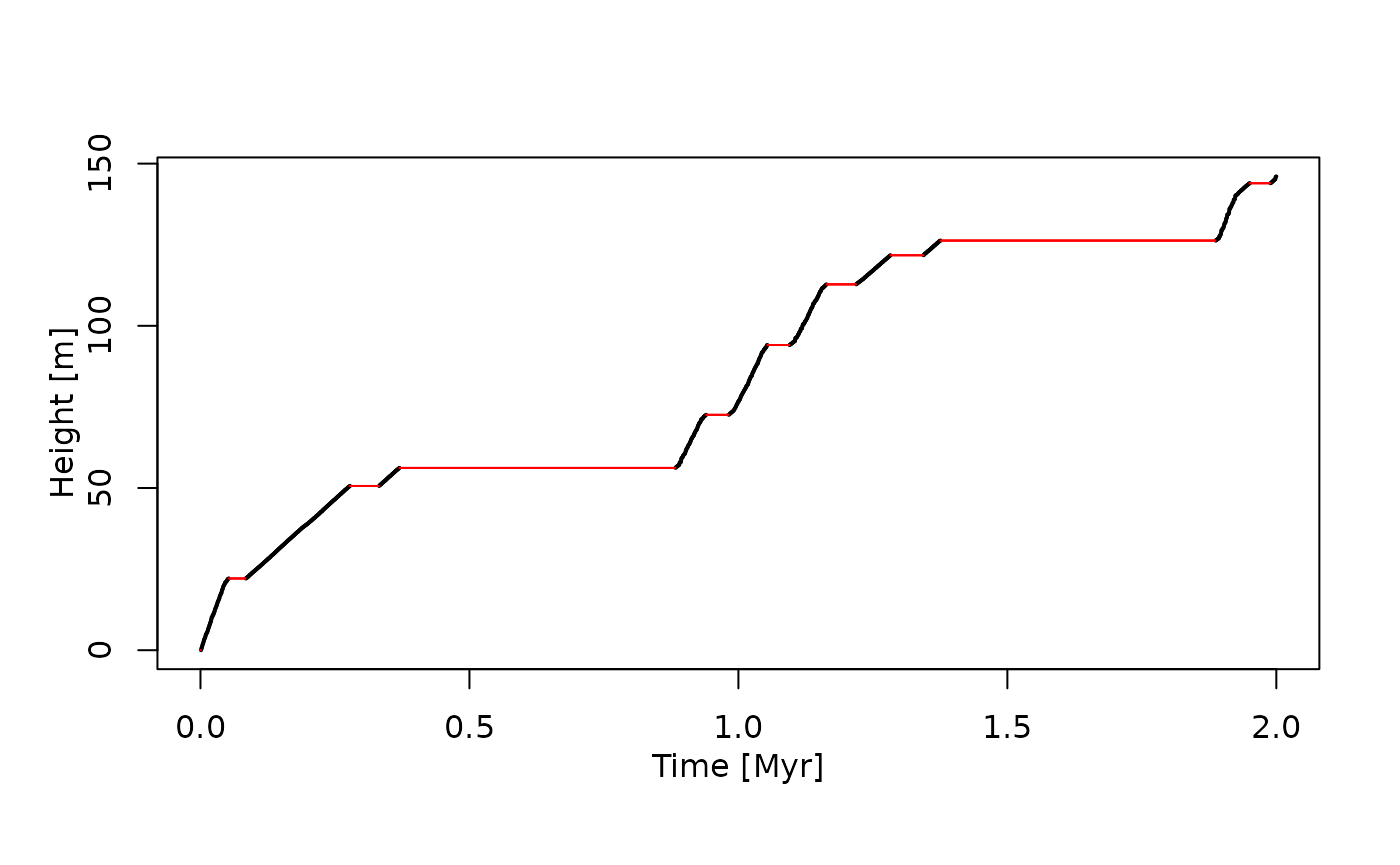

You can also plot sedimentation rates in the time domain using plot_sed_rate_t“:

plot_sed_rate_t(my_adm)

For more information on the extraction of sedimentation rates in the time domain see the functions sed_rate_t and sed_rate_t_fun. Sedimentation rates in the length domain can be extracted using sed_rate_l and sed_rate_l_fun and plotted via plot_sed_rate_l. In addition, condensation (time preserved per stratigraphic increment) can be examined using the functions condensation, condensation_fun and plot_condensation.

Extracting data from age-depth models

Use the functions get_total_duration, get_total_thickness, get_completeness, and get_hiat_no to extract information:

get_total_duration(my_adm) #total time covered by the age-depth model
#> [1] 2
get_total_thickness(my_adm) # total thickness of section represented by the adm
#> [1] 146.0621
get_completeness(my_adm) # stratigraphic completeness as proportion
#> [1] 0.3265
get_incompleteness(my_adm) # stratigraphic incompleteness (= 1- strat. incompleteness)
#> [1] 0.6735
get_hiat_no(my_adm) # number of hiatuses
#> [1] 10

For more detailed information, you can use

get_hiat_duration to get a vector of hiatus durations
get_hiat_list to get a list of hiatus positions and duration.

For example, to plot a histogram of hiatus durations, use

hist(x = get_hiat_duration(my_adm),
     freq = TRUE,
     xlab = "Hiatus duration [Myr]",
     main = "Hiatus duration 2 km offshore")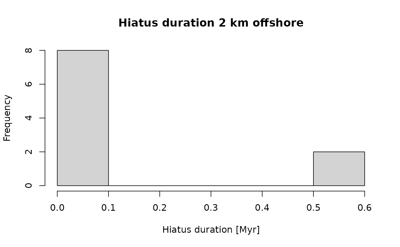

The function is_destructive can be used to examine whether points in time coincide with hiatuses:

is_destructive(my_adm,
               t = c(0.1,0.5)) 
#> [1] FALSE  TRUE

Transforming data between time and stratigraphic domain

Heights and times

The functions get_height and get_time are the workhorses to transform data using age-depth models.

get_time takes and adm object and vector of heights h (stratigraphic positions), and returns a vector of times
get_height takes an adm object and vector of times t and returns a vector of associated stratigraphic positions

As example, say we want to know the time of deposition of the following stratigraphic positions:

h = c(30,120) # stratigraphic positions
get_time(my_adm,
         h = h)
#> [1] 0.1380552 1.2704696

Conversely, to determine what parts of the section are deposited as a specific time, use

t = c(0.2,1.4)
get_height(my_adm,
           t = t)
#> [1] 39.13951       NA

Here, the NA indicates that the time 1.4 coincides with erosion. If you want to know the stratigraphic position of the hiatus that coincides with that time, use the option destructive = FALSE:

t = c(0.2,1.4)
get_height(my_adm,
           t = t,
           destructive = FALSE)
#> [1]  39.13951 126.27764

Alternatively, you can also use the wrappers strat_to_time and time_to_strat for the transformation. For expanded modeling features please use the StratPal package (Github | Webpage | CRAN). It provides more biological context and utility functions to build modeling pipelines that include ecological, taphonomic, stratigraphic, and evolutionary effects.

Phylogenetic trees

The admtools package can transform complex objects between the time and stratigraphic domain. This is done using the functions strat_to_time and time_to_strat.

As an example, we transform a chronogram (a phylogenetic tree where branch length represents time). An example tree following the birth-death model is stored with the package as the variable timetree. See ?timetree for details on how this tree was generated.

#install.packages("ape") Package for analyses of phylogenetics and evolution
# see ?ape::rlineage for help
#set.seed(1)

ape::plot.phylo(timetree) # see also ?ape::plot.phylo
axis(1)
mtext("Time [Myr]", side = 1, line = 2.5)

You can transform the tree using time_to_strat:

tree_in_strat_domain = time_to_strat(obj = timetree,
                                     x = my_adm)

Plotting the resulting tree along the stratigraphic column shows how the evolutionary relationships would be preserved 2 km offshore in the simulated carbonate platform:

ape::plot.phylo(tree_in_strat_domain, direction = "upwards")
axis(side = 2)
mtext("Stratigraphic Height [m]",
      side = 2,
      line = 2)

Lists and time/stratigraphic series

admtools can transform lists from the time to the height domain and vice versa given they have elements with names h or t. These lists can be interpreted as time/stratigraphic series, where times and stratigraphic positions are associated with measured values. Note that these are not ts objects as used by the stats package, as they will be generally heterodistant due to the irregular nature of the age-depth transformation.

As example, we simulate trait evolution over 2 Myr using a Brownian motion, and transform the simulation into the stratigraphic domain.

t = seq(0, 2, by = 0.001) # times
BM = function(t){
  #" Simulate Brownian motion at times t
  li = list("t" = t,
            "y" = cumsum(c(0, rnorm(n = length(t) - 1, mean = 0, sd = sqrt(diff(t))))))
  class(li) = c("timelist", "list") # assign class `timelist` for easy plotting, see ?plot.timelist
  return(li)
}
evo_list = BM(t)
plot(x = evo_list,
     xlab = "Time [Myr]",
     ylab = "Trait Value",
     type = "l")

strat_list = time_to_strat(obj = evo_list,
                            x = my_adm)
plot(x = strat_list,
     orientation = "lr",
     type = "l",
     xlab = "Stratigraphic Height [m]",
     ylab = "Trait Value",
     main = "Trait Evolution 2 km Offshore")

Note the jump in traits generated by the erosional interval in my_adm. Both time_to_strat and strat_to_time return stratlist and timelist objects when applied to lists. These are like ordinary lists, but come with simplified plotting optionality, see ?plot.stratlist and ?plot.timelist for details.

For expanded modeling features with biological context, please use the StratPal package (Github | Webpage | CRAN). It provides light wrappers around admtools and out of the box modeling of trait evolution.

Numeric vectors

Numeric vectors can be transformed using time_to_strat and strat_to_time too. These are essentially high level wrappers around get_height and get_time. See functions time_to_strat.numeric and strat_to_time.numeric for details.

Further information

For an overview of the structure of the admtools package and the classes used therein see

vignette("admtools_doc")

For details on plotting ADMs see

vignette("adm_plotting)

For information on estimating age-depth models from sedimentation rates, see

vignette("adm_from_sedrate")

For information on estimating age-depth models from tracer contents of rocks and sediments, see

vignette("adm_from_trace_cont")

For information on depth-depth curves and correlation see

vignette("correlation")

References

Burgess, Peter. “CarboCAT: A cellular automata model of heterogeneous carbonate strata.” Computers & geosciences 53 (2013): 129-140. DOI: 10.1016/j.cageo.2011.08.026
Burgess, Peter. “CarboCAT Lite v1.0.1”. Zenodo 2023. DOI: 10.5281/zenodo.8402578
Hohmann, Niklas; Koelewijn, Joël R.; Burgess, Peter; Jarochowska, Emilia. 2024. “Identification of the mode of evolution in incomplete carbonate successions.” BMC Ecology and Evolution 24, 113. https://doi.org/10.1186/s12862-024-02287-2.
Hohmann, Niklas, Koelewijn, Joël R.; Burgess, Peter; Jarochowska, Emilia. 2023. “Identification of the Mode of Evolution in Incomplete Carbonate Successions - Supporting Data.” Open Science Framework. https://doi.org/10.17605/OSF.IO/ZBPWA, published under the CC-BY 4.0 license.

Niklas Hohmann